Tutorial: Modeling with Cimba Python

A simple M/M/1 queue parallelized

In this section, we will walk through the development of a simple model from connecting basic entities and interactions to parallelizing the model on all available CPU cores and producing presentation-ready output.

Our first simulated system is an M/M/1 queue. In queueing theory notation, this abbreviation indicates a queueing system where the arrival process is memoryless with exponentially distributed intervals, the service process is the same, there is only one server, and the queue has unlimited capacity. This is a mathematically well understood system, which is exactly what we want for a first simulation model.

The simulation model will verify if the well-known formula for expected queue length is correct. Or, if one is feeling a bit more modest, it will verify that our model is close enough to the formula that we have probably connected the pieces correctly.

Arrival, service, and the queue

We model this in a straightforward manner. We need an arrival process that puts customers into the queue at random intervals, a service process that gets customers from the queue and services them for a random duration, and the queue itself. We are not concerned with the characteristics of each customer, just how many there are in the queue, so we do not need a separate object for each customer. We will use a sim.Queue for this.

In Cimba Python, the simulated world’s parameters, outputs, and passive simulation entities are declared as fields on a sim.Model subclass:

import cimba
import cimba.sim as sim
import cimba.random as random

class MM1(sim.Model):
    utilization: sim.Param
    avg_queue_length: sim.Output
    queue: sim.Queue

model = MM1("MM1")

utilization is a parameter supplied by the experiment. avg_queue_length is an output collected at the end of each trial. queue is a trial-local simulation queue. Each trial gets its own parameter values, output values, and queue, so trials can run independently.

Let us start with the arrival and service processes. The code can be very simple:

@model.process
def arrival(env: MM1):
    while True:
        t_ia = random.exponential(1.0 / env.utilization)
        sim.hold(t_ia)
        env.queue.put(1)

@model.process
def service(env: MM1):
    while True:
        env.queue.get(1)
        t_srv = random.exponential(1.0)
        sim.hold(t_srv)

This should hopefully be quite intuitive. The arrival process generates an exponentially distributed random value with mean 1 / utilization, holds for that amount of interarrival time, puts one new customer into the queue, and does it again.

Similarly, the service process gets a customer from the queue, waiting for one to arrive if there are none waiting, generates a random service time with mean 1.0, holds for the service time, and does it all over again. An average arrival rate of 0.75 and service rate of 1.0 gives the 0.75 utilization we wanted for the first run.

The env argument is the trial-local model record. It holds the parameter, output, state, and entity handles declared on MM1. Process functions are plain Python functions, but the blocking sim.hold() call and entity methods such as env.queue.get() make them simulation processes. If the service process tries to get from an empty queue, it pauses. The dispatcher then runs some other event, such as the arrival process waking up and putting a customer into the queue. When the service process resumes, it continues immediately after the same env.queue.get() call.

Finally, collect a time-weighted queue statistic:

@model.collect
def collect_stats(env: MM1):
    env.avg_queue_length = env.queue.mean_level()

The collector runs after the trial finishes. env.queue.mean_level() uses the recording window controlled by the experiment’s warmup and duration.

We also need an experiment to set it all up and run the simulation. Unlike a lower-level program, there is no manual object lifecycle code here: the model declaration tells Cimba Python what each trial needs, and model.experiment(...) generates the trial table.

Let us try this:

def main() -> None:
    cimba.logger_flags_on(cimba.LOGGER_INFO)
    exp = model.experiment(
        utilization=[0.75],
        replications=1,
        duration=10.0,
        warmup=0.0,
        seed=42,
    )
    failures = exp.run()
    if failures:
        raise RuntimeError(f"{failures} trial(s) failed")
    avg = float(exp["avg_queue_length"][0])
    print(f"Average queue length over the first 10 time units: {avg:.6f}")

There is one utilization value and one replication, so this experiment has one trial. The seed makes the random stream reproducible. exp.run() executes the trial table and returns the number of failed trials. Outputs are available by name, so exp["avg_queue_length"] returns an array with one element per trial.

We can now run tutorial/tut_1_1.py and see what happens. In the default release-style build used for this documentation pass, detailed internal trace logging is compiled out, so this first script prints only the collected result:

$ .venv/bin/python tutorial/tut_1_1.py
Average queue length over the first 10 time units: 0.939453

That is not a very informative run yet, but it proves that the model starts, stops, and produces an output value. We will add more useful logging and reporting shortly.

Stopping a simulation

We will address stopping first. An arrival loop and a service loop are both infinite. That is natural for many simulation processes: a server keeps serving, a weather process keeps updating, and an arrival process keeps generating work. A trial therefore needs a separate end condition.

The normal Python way is to pass duration to model.experiment(...). The generated trial starts the registered processes, opens the measurement window after warmup, closes it at warmup + duration, runs the collectors, and stops the remaining model processes. For a first model, this is both the simplest and the least surprising way to stop:

For most models, this is the cleanest stopping rule:

exp = model.experiment(
    utilization=[0.75],
    replications=1,
    duration=10.0,
    warmup=0.0,
    seed=43,
)
exp.run()

Sometimes the domain has its own stop condition: serve 100 customers, empty all work after closing time, finish a campaign, or stop when a rare event happens. Use an event callback for that:

class StopAtCount(sim.Model):
    served: sim.State
    queue: sim.Queue
    arrival: sim.Processes
    service: sim.Processes
    stop_now: sim.Event

model = StopAtCount("stop-at-count")

@model.event
def stop_now(env: StopAtCount):
    sim.stop(env.arrival[0], 0)
    sim.stop(env.service[0], 0)
    sim.clear_events()

@model.process
def monitor(env: StopAtCount):
    while env.served < 100:
        sim.hold(1.0)
    sim.schedule(env.stop_now, env, 0.0)

sim.Processes fields publish handles for registered processes. Since arrival and service each have one copy, env.arrival[0] and env.service[0] identify the running processes. sim.schedule() schedules the callback relative to the current simulation time; sim.schedule_at() schedules at an absolute time. Event handles can be cancelled, rescheduled, reprioritized, inspected, and waited on with sim.wait_event().

We run the revised program and it reaches the same 10.0 end time:

$ .venv/bin/python tutorial/tut_1_2.py
Simulation stopped at t=10.0, average queue length: 0.000000

Progress: It started, ran, and now also stopped.

Use explicit stopping sparingly. The built-in duration rule also manages the statistics window, so it is usually better for performance experiments and steady-state simulations.

Setting logging levels

Next, the verbiage. Cimba Python has logging controls that make it possible to see what is happening inside a model while it is still small enough that the trace can be read by a human.

There are two layers of logging control:

top-level logger flags, toggled with cimba.logger_flags_on() and cimba.logger_flags_off(),
and process-body helpers in cimba.sim.

The process-body helpers are intentionally simple: they log static text, integer values, or floating-point values. Register the text once, outside the process body:

import cimba
import cimba.sim as sim
import cimba.random as random

USERFLAG1 = 0x00000001

MSG_ARR_HOLD = sim.log_text("Holds for")
MSG_ARR_PUT = sim.log_text("Puts one into the queue")
MSG_SRV_GET = sim.log_text("Gets one from the queue")
MSG_SRV_HOLD = sim.log_text("Got one, services it for")

@model.process
def arrival(env: MM1):
    while True:
        t_ia = random.exponential(1.0 / env.utilization)
        sim.log_user_f64(USERFLAG1, MSG_ARR_HOLD, t_ia)
        sim.hold(t_ia)
        sim.log_user(USERFLAG1, MSG_ARR_PUT)
        env.queue.put(1)

@model.process
def service(env: MM1):
    while True:
        sim.log_user(USERFLAG1, MSG_SRV_GET)
        env.queue.get(1)
        t_srv = random.exponential(1.0)
        sim.log_user_f64(USERFLAG1, MSG_SRV_HOLD, t_srv)
        sim.hold(t_srv)

And choose the flags for the run:

cimba.logger_flags_off(cimba.LOGGER_INFO)
cimba.logger_flags_on(USERFLAG1)

We run tutorial/tut_1_3.py and get this output:

$ .venv/bin/python tutorial/tut_1_3.py
      0.0000    arrival     python (0):  Holds for 0.144672
      0.0000    service     python (0):  Gets one from the queue
     0.14467    arrival     python (0):  Puts one into the queue
     0.14467    arrival     python (0):  Holds for 0.353541
     0.14467    service     python (0):  Got one, services it for 0.285614
     0.43029    service     python (0):  Gets one from the queue
     0.49821    arrival     python (0):  Puts one into the queue
     0.49821    arrival     python (0):  Holds for 1.050368
     0.49821    service     python (0):  Got one, services it for 1.942461
      1.5486    arrival     python (0):  Puts one into the queue
      1.5486    arrival     python (0):  Holds for 1.773069
      2.4407    service     python (0):  Gets one from the queue
      2.4407    service     python (0):  Got one, services it for 0.209677
      2.6504    service     python (0):  Gets one from the queue
      3.3217    arrival     python (0):  Puts one into the queue
      3.3217    arrival     python (0):  Holds for 0.349020
      3.3217    service     python (0):  Got one, services it for 0.067436
      3.3891    service     python (0):  Gets one from the queue
      3.6707    arrival     python (0):  Puts one into the queue
      3.6707    arrival     python (0):  Holds for 0.307979
      3.6707    service     python (0):  Got one, services it for 0.185038
      3.8557    service     python (0):  Gets one from the queue
      3.9787    arrival     python (0):  Puts one into the queue
      3.9787    arrival     python (0):  Holds for 0.960811
      3.9787    service     python (0):  Got one, services it for 0.618192
      4.5968    service     python (0):  Gets one from the queue
      4.9395    arrival     python (0):  Puts one into the queue
      4.9395    arrival     python (0):  Holds for 2.020638
      4.9395    service     python (0):  Got one, services it for 0.006503
      4.9460    service     python (0):  Gets one from the queue
      6.9601    arrival     python (0):  Puts one into the queue
      6.9601    arrival     python (0):  Holds for 1.498207
      6.9601    service     python (0):  Got one, services it for 0.056081
      7.0162    service     python (0):  Gets one from the queue
      8.4583    arrival     python (0):  Puts one into the queue
      8.4583    arrival     python (0):  Holds for 0.707779
      8.4583    service     python (0):  Got one, services it for 0.452901
      8.9112    service     python (0):  Gets one from the queue
      9.1661    arrival     python (0):  Puts one into the queue
      9.1661    arrival     python (0):  Holds for 0.614626
      9.1661    service     python (0):  Got one, services it for 0.182892
      9.3490    service     python (0):  Gets one from the queue
      9.7807    arrival     python (0):  Puts one into the queue
      9.7807    arrival     python (0):  Holds for 0.825184
      9.7807    service     python (0):  Got one, services it for 2.091059
Average queue length with user logging enabled: 0.089209

Only our user-defined logging messages are printed. The simulation time, active process, and trial index are still prepended, which is exactly what we want when debugging process interactions.

Because trials may run in parallel, log lines from different trials can interleave. Logging is therefore best for short debugging runs, not for production sweeps.

Collecting and reporting statistics

Which brings us to getting some useful output. By now, we are suitably convinced that our simulated M/M/1 queue is behaving as expected, so we want it to report statistics on the queue length.

The M/M/1 formula predicts an expected waiting-queue length

\[L_q = \frac{\rho^2}{1-\rho}\]

where rho is utilization. With rho = 0.75, the expected waiting-queue length is 2.25. Short runs vary wildly, so we increase the running time from ten to one million time units and skip the first thousand time units as warmup:

exp = model.experiment(
    utilization=[0.75],
    replications=1,
    duration=1.0e6,
    warmup=1.0e3,
    seed=45,
)
failures = exp.run()
if failures:
    raise RuntimeError(f"{failures} trial(s) failed")
print(float(exp["avg_queue_length"][0]))

Time-weighted entity summaries are the right tool for levels and utilization: env.<queue>.mean_level() for queues, env.<resource>.mean_in_use() for resources, env.<pool>.mean_in_use() for pools, env.<store>.mean_length() for stores, and env.<pqueues>[i].mean_length() for priority queues. These convenience methods are shorthand for getting the entity’s recorded time series and summarizing it. For example, the following two assignments are equivalent:

@model.collect
def collect_stats(env: MM1):
    env.avg_queue_length = env.queue.mean_level()

    env.avg_queue_length = env.queue.history().mean()

The explicit history form also gives access to text reports and diagnostic plots. During a single-trial debugging run, print the queue report and a partial autocorrelation correlogram directly from the collector:

@model.collect
def collect_stats(env: MM1):
    env.avg_queue_length = env.queue.history().mean()
    env.queue.report()
    env.queue.history().pacf_correlogram(lags=20)

Very shortly thereafter, output appears. This block is from an actual run of .venv/bin/python tutorial/tut_1_4.py:

Buffer levels for queue
N  1312937  Mean    2.256  StdDev    2.850  Variance    8.123  Skewness    2.594  Kurtosis    10.26
--------------------------------------------------------------------------------
( -Infinity,      0.000)   |
[     0.000,      1.900)   |##################################################
[     1.900,      3.800)   |###############=
[     3.800,      5.700)   |#########-
[     5.700,      7.600)   |#####-
[     7.600,      9.500)   |##=
[     9.500,      11.40)   |#=
[     11.40,      13.30)   |=
[     13.30,      15.20)   |=
[     15.20,      17.10)   |-
[     17.10,      19.00)   |-
[     19.00,      20.90)   |-
[     20.90,      22.80)   |-
[     22.80,      24.70)   |-
[     24.70,      26.60)   |-
[     26.60,      28.50)   |-
[     28.50,      30.40)   |-
[     30.40,      32.30)   |-
[     32.30,      34.20)   |-
[     34.20,      36.10)   |-
[     36.10,      38.00)   |-
[     38.00,  Infinity )   |-
--------------------------------------------------------------------------------
           -1.0                              0.0                              1.0
--------------------------------------------------------------------------------
   1   0.954                                  |###############################-
   2   0.342                                  |###########-
   3  -0.173                            =#####|
   4   0.137                                  |####=
   5  -0.089                               =##|
   6   0.087                                  |##=
   7  -0.057                                =#|
   8   0.064                                  |##-
   9  -0.046                                =#|
  10   0.051                                  |#=
  11  -0.037                                -#|
  12   0.043                                  |#-
  13  -0.031                                -#|
  14   0.034                                  |#-
  15  -0.027                                 =|
  16   0.032                                  |#-
  17  -0.025                                 =|
  18   0.029                                  |=
  19  -0.022                                 =|
  20   0.025                                  |=
--------------------------------------------------------------------------------
Theory predicts an average M/M/1 waiting-queue length of 2.25
Simulation result: 2.256006

The text-mode histogram uses # for a full bar segment, = for a segment more than half full, and - for a segment that contains something but less than half a full segment. This is not publication-ready graphics, but it is surprisingly useful at the model development stage. We have numbers. Theory predicts 2.25. The run above gave 2.256006.

Close, but is it close enough? We need more resolving power.

The *_file() variants write the same text output to a path handle created with sim.log_text():

REPORT = sim.log_text("mm1_queue_report.txt")

@model.collect
def collect_stats(env: MM1):
    env.queue.report_file(REPORT, append=0)

Use stdout reports for short single-trial runs. In parallel experiments, text from several trials may interleave; prefer scalar outputs for final analysis and file reports only when each run has an unambiguous destination.

Use sim.Dataset when you need to record individual samples, such as each customer’s time in system:

class Waits(sim.Model):
    wait_mean: sim.Output
    wait_std: sim.Output
    waits: sim.Dataset

@model.process
def observer(env: Waits):
    env.waits.add(2.5)
    env.waits.add(3.0)
    sim.suspend()

@model.collect
def collect(env: Waits):
    env.wait_mean = env.waits.mean()
    env.wait_std = env.waits.std()

Datasets also provide count, minimum, and maximum. They are useful for per-agent outcomes; time-weighted summaries are useful for states that persist between event times. Datasets also have the same text-reporting style:

@model.collect
def collect(env: Waits):
    env.wait_mean = env.waits.mean()
    env.wait_std = env.waits.std()

    env.waits.fivenum()
    env.waits.histogram(bins=20)
    env.waits.correlogram(lags=20)
    env.waits.pacf_correlogram(lags=20)

Use env.waits.print() when you want the raw sample values themselves. Use env.waits.print_file(), env.waits.fivenum_file(), env.waits.histogram_file(), env.waits.correlogram_file(), and env.waits.pacf_correlogram_file() to write those reports to files.

Refactoring for parallelism

Before parallelizing, we will clean up a few rough edges. The first examples put everything at module scope. That is fine for a toy, but larger projects benefit from a builder function and from grouping repeated model structure into components. For the M/M/1 model, the queue and its two process loops form a natural station:

class MM1Station(sim.Component):
    queue: sim.Queue

    @sim.process
    def arrival(self, env):
        while True:
            t_ia = random.exponential(1.0 / env.utilization)
            sim.hold(t_ia)
            self.queue.put(1)

    @sim.process
    def service(self, env):
        while True:
            self.queue.get(1)
            t_srv = random.exponential(1.0)
            sim.hold(t_srv)


class MM1(sim.Model):
    utilization: sim.Param
    avg_queue_length: sim.Output
    station: MM1Station = MM1Station()

Component process methods are lowered into ordinary model processes before compilation. Inside the component, self.queue refers to the queue declared on the station instance. The compiled trial record remains flat, but the source code can stay grouped around the station concept.

The builder now only needs to create the model and register the collector:

def build_model() -> MM1:
    model = MM1("MM1")

    @model.collect
    def collect_stats(env: MM1):
        env.avg_queue_length = env.station.queue.mean_level()

    return model

This pattern makes it easy to write tests, command-line scripts, notebooks, and benchmarks that all build the same model. It also separates model declaration from experiment setup. Parameters and outputs belong to the trial table; component process logic belongs with the component, and experiment setup belongs outside the model.

Model callbacks can read component fields with natural dotted access such as env.station.queue. Cimba lowers that access to the flat internal field before compilation. In the experiment table, component fields still use flattened names for now, such as station__queue.

Repeated structures can be grouped the same way with standard Python list annotations:

class Attraction(sim.Component):
    queues: sim.PQueues = sim.count("queue_count")

    def __init__(self, queue_count: int, server_count: int):
        self.queue_count = queue_count
        self.server_count = server_count

    @sim.process(copies="server_count")
    def server(self, env, idx):
        q = self.queues[idx % self.queue_count]
        # serve one visitor from q ...


class Park(sim.Model):
    attractions: list[Attraction] = [
        Attraction(queue_count=1, server_count=1),
        Attraction(queue_count=3, server_count=3),
    ]

Model callbacks can index the collection with env.attractions[i].queues[j]. Cimba lowers that to flattened fields and generated offset arrays; experiment fields still use names such as attractions__queues and attractions__server_state.

Components can also contain other components. This is useful when a natural object has smaller named parts:

class RideQueues(sim.Component):
    line: sim.PQueues = sim.count("queue_count")

    def __init__(self, queue_count: int):
        self.queue_count = queue_count


class RideServers(sim.Component):
    served: sim.State


class Attraction(sim.Component):
    queues: RideQueues
    servers: RideServers

    def __init__(self, queue_count: int, server_count: int):
        self.queues = RideQueues(queue_count)
        self.servers = RideServers()
        self.server_count = server_count

    @sim.process(copies="server_count")
    def server(self, env, idx):
        q = self.queues.line[idx % self.queues.queue_count]
        self.servers.served += 1
        # serve one visitor from q ...

Nested fields use the same flattened public naming convention: env.attractions[i].queues.line[j] is stored under attractions__queues__line.

def run_mm1_trial(
    *,
    rho: float,
    duration: float,
    warmup: float,
    seed: int,
) -> float:
    exp = build_model().experiment(
        utilization=[rho],
        replications=1,
        duration=duration,
        warmup=warmup,
        seed=seed,
    )
    failures = exp.run()
    if failures:
        raise RuntimeError(f"{failures} trial(s) failed")
    return float(exp["avg_queue_length"][0])

Parallelization

So far, we have been developing the model as if it were a single run. The simulation is already fast, but a modern CPU has many cores, most of them idly watching our work so far with detached interest. Let’s put them to work.

Parallelizing a single simulated world is hard because the outcome of one event may influence all future events. Parallelizing an experiment is much easier. We rarely want only one run. We want many replications, many parameter combinations, or both. These trials are designed to be independent, so they can run at the same time.

In Cimba Python, parallel experiments are just larger trial tables. Parameter values are arrays, and replications repeats every parameter combination:

import numpy as np

rhos = np.arange(0.025, 1.0, 0.025)
replications = 10

exp = build_model().experiment(
    utilization=rhos,
    replications=replications,
    duration=1.0e6,
    warmup=1.0e3,
    seed=42,
)
failures = exp.run()
if failures:
    raise RuntimeError(f"{failures} trial(s) failed")

values = exp["avg_queue_length"].reshape(len(rhos), replications)

When the run is finished, summarize each row:

print(f"{'rho':>8} {'simulated':>10} {'+/-95%':>10} {'theory':>10}")
for rho, samples in zip(rhos, values):
    mean = float(samples.mean())
    ci = float(1.96 * samples.std(ddof=1) / np.sqrt(samples.size))
    theory = rho * rho / (1.0 - rho)
    print(f"{rho:8.3f} {mean:10.4f} {ci:10.4f} {theory:10.4f}")

tutorial/tut_1_7.py is the command-line version. It accepts replication count, duration, warmup, seed, and an optional timing flag. The shorter tutorial/tut_1_6.py script prints this table:

$ .venv/bin/python tutorial/tut_1_6.py
cimba 3.0.0-beta
     rho  simulated     +/-95%     theory
025     0.0006     0.0000     0.0006
050     0.0026     0.0001     0.0026
075     0.0061     0.0001     0.0061
100     0.0111     0.0001     0.0111
125     0.0177     0.0002     0.0179
150     0.0266     0.0002     0.0265
175     0.0371     0.0002     0.0371
200     0.0500     0.0004     0.0500
225     0.0651     0.0003     0.0653
250     0.0832     0.0004     0.0833
275     0.1046     0.0007     0.1043
300     0.1284     0.0007     0.1286
325     0.1559     0.0011     0.1565
350     0.1892     0.0008     0.1885
375     0.2257     0.0007     0.2250
400     0.2680     0.0014     0.2667
425     0.3143     0.0013     0.3141
450     0.3674     0.0013     0.3682
475     0.4294     0.0016     0.4298
500     0.4989     0.0020     0.5000
525     0.5800     0.0027     0.5803
550     0.6712     0.0031     0.6722
575     0.7789     0.0035     0.7779
600     0.9024     0.0047     0.9000
625     1.0417     0.0068     1.0417
650     1.2059     0.0059     1.2071
675     1.3928     0.0068     1.4019
700     1.6293     0.0071     1.6333
725     1.9034     0.0115     1.9114
750     2.2564     0.0156     2.2500
775     2.6621     0.0205     2.6694
800     3.2082     0.0303     3.2000
825     3.8639     0.0318     3.8893
850     4.8088     0.0638     4.8167
875     6.1282     0.0778     6.1250
900     8.0668     0.1274     8.1000
925    11.3918     0.2103    11.4083
950    18.1704     0.2903    18.0500
975    41.5860     1.8192    38.0250

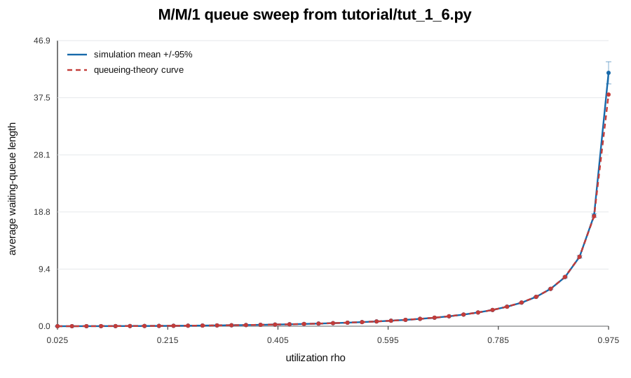
Evidently, we cannot reject the hypothesis that conventional queueing theory may be correct. Nor can we reject the hypothesis that Cimba Python may be working correctly.

The plot below was generated from that same run, using tutorial/tut_1_6.py data and a small SVG writer:

This concludes the first tutorial. We have followed the development steps from a first minimal model demonstrating process interactions to a complete parallelized experiment with summarized output. The files tutorial/tut_1_*.py include working code for each stage of development.

Acquiring, preempting, holding, and releasing resources, with interruptions

We will now introduce ways of acquiring and releasing resources of various kinds. We will also show additional process interactions where one active process acts directly on another process. We will demonstrate these through a somewhat cartoonish example, but first we need a little background.

Resources and resource pools

Cimba Python provides two kinds of resources that a process can acquire, hold, and release. sim.Resource is a single exclusive unit, while sim.Pool is a collection of interchangeable units. In computer science terms, the first is a binary semaphore and the second is a counting semaphore.

If the requested resource or number of pool units is not available, the acquire call waits in priority order. The ordering is determined first by process priority, then by arrival order among processes with the same priority. Changing a process priority with sim.set_priority() also affects its place in waiting queues.

The typical usage pattern is also the reason the time-delay function is called sim.hold():

class Shop(sim.Model):
    station: sim.Resource
    tools: sim.Pool = 8

model = Shop("shop")

@model.process
def job(env: Shop):
    station_sig = env.station.acquire()
    if station_sig != sim.SUCCESS:
        return

    tool_sig = env.tools.acquire(3)
    if tool_sig == sim.SUCCESS:
        sim.hold(5.0)
        env.tools.release(3)

    env.station.release()

Or, for a pool:

@model.process
def job(env: Shop):
    sig = env.tools.acquire(6)
    if sig == sim.SUCCESS:
        sim.hold(2.0)
        env.tools.release(3)
        sim.hold(1.0)
        env.tools.release(3)

Note that resources and pools are different from count queues. It is meaningful to put 100 items into a queue with capacity 10; the process can fill the queue, wait for space, and continue until all 100 are in. It is not meaningful to acquire 11 units from a pool whose maximum capacity is 10. That model request cannot ever be satisfied, so it should be treated as a model error.

The return value matters. A process may wake because the request succeeded, but it may also wake because it was interrupted, stopped, timed out, cancelled, or preempted. The common signal constants are sim.SUCCESS, sim.PREEMPTED, sim.INTERRUPTED, sim.STOPPED, sim.CANCELLED, and sim.TIMEOUT.

Pool accounting should be read from the pool when correctness matters:

me = sim.current()
held = env.tools.held(me)
available = env.tools.available()
in_use = env.tools.in_use()

This is especially important when preemption is possible. A process can lose capacity while blocked in a different call, so a local variable that says “I think I hold 4 units” should be resynchronized with env.tools.held() after any blocking operation.

Preemptions and interruptions

A yielded process does not have any guarantees about what may happen before it resumes control. Other processes may act on it, perhaps stopping it outright, waking it up early, or taking away resources it is holding. To tell these cases apart, blocking process and resource calls return integer signals.

Preemption is a resource-pool operation: a higher-priority process can take capacity away from lower-priority holders. Interruption is process-directed: a process handle is woken with a signal.

class Crew(sim.Model):
    worker: sim.Processes = 4
    tools: sim.Pool = 10
    interrupted: sim.State
    preempted: sim.State

model = Crew("crew")

@model.process(copies=4)
def worker(env: Crew, idx: int):
    me = sim.current()
    held = 0
    while True:
        sim.set_priority(me, idx)
        sig = env.tools.acquire(4)
        held = env.tools.held(me)
        if sig == sim.PREEMPTED:
            env.preempted += 1
        elif sig != sim.SUCCESS:
            env.interrupted += 1

        sig = sim.hold(100.0)
        held = env.tools.held(me)
        if sig == sim.PREEMPTED:
            env.preempted += 1
        elif sig != sim.SUCCESS:
            env.interrupted += 1

        if held:
            env.tools.release(held)

@model.process
def supervisor(env: Crew):
    sim.hold(1.0)
    sim.interrupt(env.worker[0], sim.INTERRUPTED, 0)
    env.tools.preempt(6)

The supervisor uses the process handles published by env.worker. In a real model this could be an emergency dispatcher interrupting a crew, a maintenance controller stopping a machine, or a triage process changing a patient’s path.

There are several possible outcomes when a process is waiting for more capacity:

The request succeeds and the call returns sim.SUCCESS.
A higher-priority process preempts capacity and the waiting process wakes with sim.PREEMPTED.
Another process interrupts it with sim.interrupt(), and the call returns the signal value chosen by the interrupter.

This is why the example checks both the return signal and the amount still held. Signals explain why the process woke. Entity queries such as env.tools.held() tell the process what the simulated world looks like now.

Buffers and object queues, interrupted

The semantics of queues and stores are different from resources. A process can hold a resource, making it unavailable until released. Queue contents are not held in the same sense: once an item is put in, another process may get it and consume it immediately.

sim.Queue stores counts. sim.Store stores integer payloads. sim.PQueues stores integer payloads ordered by priority. All of them can block, so the same signal discipline applies.

class Inbox(sim.Model):
    jobs: sim.Store = 10
    completed: sim.State

model = Inbox("inbox")

@model.process
def producer(env: Inbox):
    for job_id in range(100):
        sig = env.jobs.put(job_id)
        if sig != sim.SUCCESS:
            return

@model.process
def consumer(env: Inbox):
    while True:
        status, job_id = env.jobs.get()
        sim.hold(1.0 + job_id % 3)
        env.completed += 1

Use env.<store>.take() when a process needs a specific payload, not simply the next available one. Priority queue elements (indexed with env.<pqueues>[i]) add .put(), .get(), .take(), .position(), .reprioritize(), and .cancel().

While the cat is away…

It is again probably easier to demonstrate with code than explain in abstract terms how all this works.

Imagine a pile of reusable capacity. Several polite agents repeatedly acquire some amount, hold it for a while, and release part or all of it. A few more aggressive agents use preemption instead. A controller sleeps most of the time, but occasionally wakes and interrupts a random active process. The interactions can get intricate, which is exactly why this makes a good stress test.

In Python, represent the agents as process copies and use process arrays for targeting:

class Game(sim.Model):
    polite: sim.Processes = 5
    aggressive: sim.Processes = 2
    resource: sim.Pool = 20
    controller_actions: sim.State

model = Game("game")

@model.process(copies=5)
def polite(env: Game):
    me = sim.current()
    while True:
        amount = random.dice(1, 5)
        sim.set_priority(me, random.dice(-10, 10))
        sig = env.resource.acquire(amount)
        if sig == sim.SUCCESS:
            sim.hold(random.exponential(1.0))
            held = env.resource.held(me)
            if held:
                env.resource.release(random.dice(1, held))

@model.process(copies=2)
def aggressive(env: Game):
    me = sim.current()
    while True:
        amount = random.dice(3, 10)
        sim.set_priority(me, random.dice(-5, 15))
        env.resource.preempt(amount)
        sim.hold(random.exponential(1.0))

@model.process
def controller(env: Game):
    while True:
        sim.hold(random.exponential(5.0))
        if random.bernoulli(0.5) == 1:
            target = env.polite[random.dice(0, 4)]
        else:
            target = env.aggressive[random.dice(0, 1)]
        sim.interrupt(target, sim.INTERRUPTED, 0)
        env.controller_actions += 1

The lesson is not the particular story. The lesson is that handles let one process act on another, and signals let the target process learn why it woke.

The runnable version in tutorial/tut_2_1.py tallies the outcomes instead of printing every step. A typical run reports averages like this:

$ .venv/bin/python tutorial/tut_2_1.py
cimba 3.0.0-beta, using 16 worker threads
5 mice and 2 rats compete for 20 cheese cubes, 1 cat chases the rodents
10 trials of 100000 time units in 0.15 s, 0 failed

              grabbed     stolen  preempted interrupted
      mice     366108     166020      67314       14501
      rats     358075     107176      16537        5566

cat chases: 28544 per trial
cheese in use: 18.9 of 20 cubes on average
accounting errors (held vs pool_held): 0

The exact names in the example are deliberately less important than the accounting result. Even under heavy preemption and interruption, the resource pool’s record of who holds what remains consistent.

Real world uses

The example above is intentionally frantic. We want to exercise many possible interleavings of acquire, preempt, hold, release, and interrupt calls. Real models will usually be calmer, but the same mechanisms are important in a wide range of applications:

staff shared across patient classes,
repair crews preempted by urgent failures,
transport vehicles interrupted by dispatch decisions,
machines that lose capacity while jobs are waiting,
berths, chargers, runways, or rooms allocated by priority.

When the model can be interrupted, write process code as a sequence of recoverable states. After each blocking call, inspect the signal and ask the entity what it still holds before deciding the next action.

This completes the second tutorial, demonstrating how to acquire and release resources, and how to use direct process interactions like sim.interrupt() and env.<pool>.preempt(). We also mentioned, but did not dwell on, sim.wait_process() and sim.wait_event(). Those are waiting tools for joining another process or waiting on a scheduled event handle.

Agents balking, reneging, and jockeying in queues

In our first tutorial, we modeled an M/M/1 queue as a simple count. That was sufficient to calculate queue length statistics. We now extend this to a more realistic and analytically intractable case where the customers are active, opinionated agents in their own right.

The customers generated by the arrival process will make their own decisions on whether to join a queue or not (balking), leave midway (reneging), or switch to another queue that seems to be moving faster (jockeying). Or patiently wait until they get served and then leave for new adventures.

The use case is an amusement park with guests wanting to use various attractions, where the park operator wants us to analyze ways of influencing customer behavior. The overall metric is the time spent in the park per visitor and the breakdown of this time between riding, waiting, and walking. The time unit is minutes.

Process-local state with sim.Struct

The object-oriented paradigm is very natural for simulation modeling. In Python, we use a sim.Struct subclass when each process instance needs its own fields: entry time, priority, patience, current queue, time spent walking, time spent waiting, and so on.

class Visitor(sim.Struct):
    patience: float
    priority: int
    entry_park: float
    entry_queue: float
    riding: float
    waiting: float
    walking: float
    rides: int

class VisitorFlow(sim.Component):
    visitor: sim.Spawnable
    departed: sim.Store
    d_park: sim.Dataset
    d_rides: sim.Dataset

We will combine this visitor-flow component with the attraction components shortly.

A sim.Component is an authoring-time grouping for related declarations and process methods. It is not a separate runtime object inside the compiled trial record. Instead, Cimba lowers component fields into ordinary flat fields before compilation. That means we can write model code in the natural domain shape (env.flow.d_park or env.attractions[i].queues.line[j]) while the compiled data layout stays simple and fast.

Components are useful when a concept has both state and behavior. In this example, VisitorFlow owns the visitor lifecycle: arrivals, dynamic visitor processes, departure cleanup, counters, and datasets. The attractions will form a component collection because the park has several repeated ride stations with the same structure but different constants.

sim.Spawnable means visitor processes are created dynamically. The arrival process spawns a new visitor and initializes its fields before the visitor first runs:

class VisitorFlow(sim.Component):
    visitor: sim.Spawnable

    @sim.process
    def arrivals(self, env):
        while True:
            sim.hold(random.exponential(2.0))
            handle = sim.spawn(self.visitor, env, priority=0)
            vip = Visitor(handle)
            vip.entry_park = sim.now()
            vip.patience = random.triangular(0.5, 1.0, 1.5)
            vip.priority = 5 if random.bernoulli(0.25) else 0

The visitor process receives its own view as the final annotated parameter on the component method:

class VisitorFlow(sim.Component):
    visitor: sim.Spawnable

    @sim.process
    def visitor(self, env, vip: Visitor):
        me = sim.current()
        vip.entry_queue = sim.now()
        q = env.attractions[0].queues.line[0]
        entry = q.put(me, vip.priority)
        sig = sim.suspend()
        if sig == sim.SUCCESS:
            vip.rides += 1

Here, self.visitor is the component-owned spawnable field, while the ride queues live on the attraction components. Model callbacks and component processes can still use natural dotted paths such as env.attractions[0].queues.line[0]; Cimba lowers those paths to the flat trial record before compilation.

The same pattern is useful for the whole visitor lifecycle. The component owns arrival generation, visitor behavior, departure cleanup, counters, and datasets:

class VisitorFlow(sim.Component):
    balks: sim.State
    jockeys: sim.State
    reneges: sim.State

    visitor: sim.Spawnable
    departed: sim.Store
    d_park: sim.Dataset
    d_riding: sim.Dataset
    d_waiting: sim.Dataset
    d_walking: sim.Dataset
    d_rides: sim.Dataset

    @sim.process
    def arrivals(self, env):
        # spawn visitors until closing time
        ...

    @sim.process
    def visitor(self, env, vip: Visitor):
        # walk, queue, balk, renege, jockey, ride, and leave
        ...

    @sim.process
    def departures(self, env):
        while True:
            sim.despawn(self.departed.take())

Another process can use Visitor(handle) to view and update the same fields. That is how a ride server records waiting and riding time for the visitor it has just taken from a priority queue. In other words, the visitor is both an active process and a small object carrying its own attributes and accumulated statistics.

The ride servers belong naturally to attractions. Each attraction owns its priority queues and starts one server process copy per physical ride server:

RideQueues is a nested component. It gives the queue group its own name inside an Attraction instead of leaving every queue field directly on the top-level model. Attraction then uses a component process method for the server loop. Inside that method, self.queues.line[...] refers to the queues of this attraction instance, and self.batch_size or self.dmin are per-attraction primitive constants captured from __init__.

class RideQueues(sim.Component):
    line: sim.PQueues = sim.count("queue_count")

    def __init__(self, queue_count: int):
        self.queue_count = queue_count


class Attraction(sim.Component):
    queues: RideQueues

    def __init__(self, attraction: int):
        self.queue_count = int(NUM_QUEUES[attraction])
        self.servers_per_q = int(SERVERS_PER_Q[attraction])
        self.server_count = self.queue_count * self.servers_per_q
        self.batch_size = int(BATCH_SIZES[attraction])
        self.dmin = float(MIN_DUR[attraction])
        self.dmode = float(MODE_DUR[attraction])
        self.dmax = float(MAX_DUR[attraction])
        self.queues = RideQueues(self.queue_count)

    @sim.process(copies="server_count")
    def server(self, env, idx: int):
        q = self.queues.line[idx // self.servers_per_q]
        riders = np.empty(MAX_BATCH, dtype=np.int64)

        while True:
            riders[0] = q.take()
            cnt = 1
            while q.length() > 0 and cnt < self.batch_size:
                riders[cnt] = q.take()
                cnt += 1

            boarding = sim.now()
            for i in range(cnt):
                sim.timers_clear(riders[i])
                vip = Visitor(riders[i])
                vip.waiting += boarding - vip.entry_queue

            dur = random.pert(self.dmin, self.dmode, self.dmax)
            sim.hold(dur)

            for i in range(cnt):
                Visitor(riders[i]).riding += dur
                sim.resume(riders[i], sim.SUCCESS)

The top-level model is now mostly composition:

The list annotation below creates a component collection. Cimba instantiates one lowered process namespace for the collection, so the nine attraction templates share an indexed process such as attractions__server. Their queue arrays are stored together, and source code can still index them by attraction.

class Park(sim.Model):
    avg_rides: sim.Output
    avg_time_in_park: sim.Output
    avg_riding: sim.Output
    avg_waiting: sim.Output
    avg_walking: sim.Output
    n_visitors: sim.Output
    n_balks: sim.Output
    n_jockeys: sim.Output
    n_reneges: sim.Output

    flow: VisitorFlow = VisitorFlow()
    attractions: list[Attraction] = [
        Attraction(attraction)
        for attraction in range(1, NUM_ATTRACTIONS + 1)
    ]

Notice the flow of control here. The visitor does not call a ride function. The visitor suspends while waiting in the queue. The server later resumes the visitor when the ride is finished. This is a very natural way to write service systems where one process batches or coordinates other processes.

Setting and clearing timers

Timers are process-specific wakeups. They are a natural way to model impatience. The visitor enters a priority queue, sets one timer for considering jockeying, sets another timer for reneging, and then suspends. It will wake when one of three things happens: the jockeying timer fires, the reneging timer fires, or a server boards it and resumes it.

TIMER_JOCKEYING = 17
TIMER_RENEGING = 42

class VisitorFlow(sim.Component):
    @sim.process
    def visitor(self, env, vip: Visitor):
        me = sim.current()
        q = env.attractions[0].queues.line[0]
        entry = q.put(me, vip.priority)

        sim.timer_add(me, vip.patience * 5.0, TIMER_JOCKEYING)
        sim.timer_add(me, vip.patience * 10.0, TIMER_RENEGING)

        while True:
            sig = sim.suspend()
            if sig == TIMER_JOCKEYING:
                my_pos = q.position(entry)
                # If another queue is shorter, cancel and re-enter there.
            elif sig == TIMER_RENEGING:
                q.cancel(entry)
                sim.timers_clear(me)
                return
            else:
                sim.timers_clear(me)
                vip.rides += 1
                return

sim.timer_set() schedules an absolute timer, sim.timer_add() schedules a relative timer, sim.timer_cancel() cancels one timer, and sim.timers_clear() clears every timer for the process. Clear timers when a process boards the ride so stale impatience events do not wake it later.

The code above omitted the actual jockeying decision. In the full model, the visitor compares its current queue position to the shortest queue at the same attraction. If another queue is shorter, it cancels its old queue entry and enters the better queue with slightly higher priority:

if sig == TIMER_JOCKEYING:
    my_pos = q.position(entry)
    new_q = env.attractions[ride].queues.line[0]
    new_len = new_q.length()
    for candidate in range(1, env.attractions[ride].queues.queue_count):
        candidate_q = env.attractions[ride].queues.line[candidate]
        candidate_len = candidate_q.length()
        if candidate_len < new_len:
            new_q = candidate_q
            new_len = candidate_len

    if new_len < my_pos:
        q.cancel(entry)
        q = new_q
        entry = q.put(me, vip.priority + 1)
        self.jockeys += 1

If the reneging timer fires, the visitor cancels the queue entry and goes somewhere else:

elif sig == TIMER_RENEGING:
    q.cancel(entry)
    sim.timers_clear(me)
    self.reneges += 1
    break

And if the signal is neither timer, the visitor was resumed by the ride server, so the ride has happened and the visitor can choose a new destination:

else:
    vip.rides += 1
    break

Alias sampling probabilities

Queueing networks often use a transition matrix: after each attraction, choose the next attraction according to row-specific probabilities. Cimba Python provides probability-based draws with cimba.random.categorical(), imported below as random.categorical().

NEXT_FROM_ENTRANCE = (0.30, 0.20, 0.20, 0.10, 0.05, 0.05, 0.10)

class VisitorFlow(sim.Component):
    @sim.process
    def visitor(self, env, vip: Visitor):
        next_stop = random.categorical(NEXT_FROM_ENTRANCE)

For a large transition matrix, keep arrays at module scope and index into the appropriate row from helper functions. Fixed arrays outside the process loop make the model easier to audit and keep the hot path clean.

In the runnable tutorial, the helper samples the row explicitly:

@njit
def _next_attraction(attraction: int) -> int:
    r = random.uniform()
    acc = 0.0
    for j in range(NUM_ATTRACTIONS + 2):
        acc += TRANSITION_PROBS[attraction, j]
        if r < acc:
            return j
    return IDX_EXIT

The row values still represent the same thing: “given where the visitor is now, where do they go next?” Whether the implementation uses cimba.random.categorical() or an explicit cumulative scan, the model concept is a weighted routing decision.

A day in the park

The complete park model has three process groups:

flow spawns visitors, runs each visitor’s day, and despawns departures,
attractions run the ride servers,
attractions[].queues connect visitors waiting for rides to the servers that board them.

The visitor’s journey is a good example of process-oriented modeling. The process reads like the entity’s day:

choose the next attraction,
walk there,
inspect the shortest queue,
balk if it is too long,
enter a priority queue and arm timers,
wake because of jockeying, reneging, or boarding,
repeat until leaving the park,
tally final statistics and hand the process handle to a cleanup process.

Finished dynamic processes should be reclaimed during long trials:

class VisitorFlow(sim.Component):
    @sim.process
    def departures(self, env):
        while True:
            sim.despawn(self.departed.take())

    @sim.process
    def visitor(self, env, vip: Visitor):
        # ... after the visitor decides to leave ...
        self.d_park.add(sim.now() - vip.entry_park)
        self.d_rides.add(1.0 * vip.rides)
        self.departed.put(sim.current())

The model can then report average time in park, rides per visitor, waiting time, walking time, balks, reneges, and jockeys. A typical run of tutorial/tut_3_1.py produces a compact table over replicated park days:

$ .venv/bin/python tutorial/tut_3_1.py
cimba 3.0.0-beta, using 16 worker threads
9 attractions, 11 queues, 14 ride servers; 960 min park day
20 trials in 0.05 s, 0 failed

per-visitor averages      mean  +/-95%
visitors / day             482   12.13
rides taken               2.71    0.03
time in park (min)        58.8    0.55
  riding                  18.7    0.22
  waiting in queues        4.8    0.20
  walking                 33.5    0.19
balks / day                  0    0.00
jockey moves / day          81    3.78
reneges / day              100    8.06

The same pattern works for clinics, call centers, airports, warehouses, and transit hubs. The story changes, but the modeling elements remain active agents, queues, priorities, timers, and recorded outcomes.

This concludes the third tutorial. We started with a queue length and ended with active agents carrying their own state, making queueing decisions, waking from timers, and being resumed by servers. That is a large conceptual step, but the Python code remains close to the story we are trying to tell.

A LNG tanker harbor with complex resources and conditions

Once upon a time, harbor simulations with ships and tugs were a natural showcase for process-oriented simulation. They still are. A harbor has active entities, scarce resources, environmental processes, and operational rules that are easy to state in words but awkward to reduce to a closed-form equation.

In this tutorial we combine several ideas: dynamic ships, environmental processes, resource pools, exclusive resources, datasets, text reports, and condition variables. Ships arrive offshore and wait until the water is deep enough, the wind is calm enough, an appropriate berth is available, and enough tugs are free. Then they dock, unload, and later depart under another tug movement.

An empty simulation template

As always, start smaller than the final ambition. Begin with a model declaration and one idle process. This is a useful sanity check before the real model grows:

class Harbor(sim.Model):
    completed: sim.Output
    ships_done: sim.State

harbor = Harbor("harbor")

@harbor.process
def placeholder(env: Harbor):
    sim.suspend()

exp = harbor.experiment(replications=1, duration=24.0, warmup=0.0, seed=1)
exp.run()

At this point you know the package imports, the model registers, and a trial can start and stop. That is not much of a harbor yet, but a boring successful run is better than an exciting broken one.

Processes, resources, and conditions

The harbor has parameters, outputs, environmental state, resources, conditions, and dynamic ships. Components let the model declaration become the table of contents for the simulated world:

class SeaConditions(sim.Component):
    wind_mag: sim.FloatState
    wind_dir: sim.FloatState
    water_depth: sim.FloatState


class HarborFacilities(sim.Component):
    tugs: sim.Pool = sim.capacity("num_tugs")
    berths_small: sim.Pool = sim.capacity("num_berths_small")
    berths_large: sim.Pool = sim.capacity("num_berths_large")
    comms: sim.Resource
    harbormaster: sim.Condition


class ShipTraffic(sim.Component):
    ship: sim.Spawnable
    departed: sim.Store
    time_small: sim.Dataset
    time_large: sim.Dataset


class Harbor(sim.Model):
    mean_wind: sim.Param
    reference_depth: sim.Param
    arrival_rate: sim.Param
    percent_large: sim.Param
    num_tugs: sim.Param
    num_berths_small: sim.Param
    num_berths_large: sim.Param

    avg_time_small: sim.Output
    avg_time_large: sim.Output
    tug_util: sim.Output

    harbormaster_called: sim.Predicate

    sea: SeaConditions = SeaConditions()
    facilities: HarborFacilities = HarborFacilities()
    traffic: ShipTraffic = ShipTraffic()

sim.capacity("num_tugs") means each trial sizes the pool from that parameter value. This lets one experiment sweep infrastructure choices without rewriting the model. The same idea is used for small and large berths. The fields still compile into the flat trial record, but source code can use paths such as env.facilities.tugs and env.sea.water_depth.

Conditions combine a wait list with a predicate:

@harbor.predicate
def harbormaster_called(env: Harbor) -> bool:
    return True

class SeaConditions(sim.Component):
    water_depth: sim.FloatState

    @sim.process
    def tide(self, env):
        while True:
            self.water_depth = env.reference_depth + random.normal(0.0, 0.5)
            env.facilities.harbormaster.signal()
            sim.hold(1.0)

The predicate above simply says “wake and recheck your own detailed rules.” That is a practical pattern when each waiting ship has different limits. A small ship and a large ship do not require the same water depth, wind limit, berth type, or number of tugs, so the detailed readiness test belongs with the ship.

Building our ships

Ships are dynamic processes with per-ship fields. A ship needs to remember what kind of ship it is, how many tugs it needs, what weather limits it can tolerate, and when it arrived:

SMALL = 0
LARGE = 1
TUGS_NEEDED = (1, 3)
MAX_WIND = (10.0, 12.0)
MIN_DEPTH = (8.0, 13.0)

class Ship(sim.Struct):
    size: int
    tugs_needed: int
    max_wind: float
    min_depth: float
    arrival: float

class ShipTraffic(sim.Component):
    ship: sim.Spawnable

    @sim.process
    def arrivals(self, env):
        mean_interarrival = 1.0 / env.arrival_rate
        while True:
            sim.hold(random.exponential(mean_interarrival))
            handle = sim.spawn(self.ship, env, 0)
            shp = Ship(handle)
            shp.size = random.bernoulli(env.percent_large)
            shp.tugs_needed = TUGS_NEEDED[shp.size]
            shp.max_wind = MAX_WIND[shp.size]
            shp.min_depth = MIN_DEPTH[shp.size]
            shp.arrival = sim.now()

The spawned process starts when the current process next blocks, so the arrival process can initialize the ship fields immediately after sim.spawn(). This is a useful pattern whenever dynamically created agents need attributes before they begin acting.

Weather and tides

Environmental processes update shared state on their own schedules. In the harbor model, wind updates first each hour and tide reads the current wind when computing water depth:

class SeaConditions(sim.Component):
    wind_mag: sim.FloatState
    water_depth: sim.FloatState

    @sim.process(priority=1)
    def weather(self, env):
        while True:
            wmag = random.rayleigh(env.mean_wind)
            self.wind_mag = 0.5 * wmag + 0.5 * self.wind_mag
            sim.hold(1.0)

    @sim.process
    def tide(self, env):
        while True:
            self.water_depth = env.reference_depth + random.normal(0.0, 0.5)
            env.facilities.harbormaster.signal()
            sim.hold(1.0)

Priorities matter when events happen at the same simulated time. Giving weather a higher priority means the hourly weather update happens before the tide process samples the state. This kind of ordering is often easier to make explicit than to hide in clever code.

Resources and condition variables

A ship can dock only if enough water is available, wind is acceptable, one berth of the right size is free, and enough tugs are available. In the componentized model, the ship process can read those domains through env.sea and env.facilities:

class ShipTraffic(sim.Component):
    @sim.process
    def ship(self, env, shp: Ship):
        if shp.size == LARGE:
            berths = env.facilities.berths_large
        else:
            berths = env.facilities.berths_small

        while True:
            ready = (
                env.sea.water_depth >= shp.min_depth
                and env.sea.wind_mag <= shp.max_wind
                and env.facilities.tugs.available()
                    >= shp.tugs_needed
                and berths.available() >= 1
            )
            if ready:
                break
            env.facilities.harbormaster.wait_for(env.harbormaster_called)

        berths.acquire(1)
        env.facilities.tugs.acquire(shp.tugs_needed)

The loop is intentional. Several ships may wake from the same signal, and one of them may take the last berth or tug before another resumes. The second ship must recheck the condition and wait again. This is not a bug; it is exactly the kind of race between simulated entities that the model should represent.

The life of a ship

The complete ship process is a readable itinerary. It waits offshore, acquires a berth and tugs, uses the radio channel to announce movement, moves in, releases the tugs while unloading, acquires them again to depart, releases the berth, records its time in system, and finally hands itself to the cleanup process.

class ShipTraffic(sim.Component):
    time_small: sim.Dataset
    time_large: sim.Dataset
    departed: sim.Store

    @sim.process
    def ship(self, env, shp: Ship):
        me = sim.current()
        if shp.size == LARGE:
            berths = env.facilities.berths_large
        else:
            berths = env.facilities.berths_small

        # ... wait until env.sea and env.facilities say docking is ready ...

        berths.acquire(1)
        env.facilities.tugs.acquire(shp.tugs_needed)

        env.facilities.comms.acquire()
        sim.hold(random.gamma(5.0, 0.01))
        env.facilities.comms.release()

        sim.hold(random.pert(0.4, 0.5, 0.8))
        env.facilities.tugs.release(shp.tugs_needed)
        env.facilities.harbormaster.signal()

        unload_avg = env.unload_avg_large if shp.size == LARGE \
            else env.unload_avg_small
        sim.hold(random.pert(0.75 * unload_avg, unload_avg,
                          2.0 * unload_avg))

        env.facilities.tugs.acquire(shp.tugs_needed)
        env.facilities.comms.acquire()
        sim.hold(random.gamma(5.0, 0.01))
        env.facilities.comms.release()
        sim.hold(random.pert(0.4, 0.5, 0.8))

        berths.release(1)
        env.facilities.tugs.release(shp.tugs_needed)
        env.facilities.harbormaster.signal()

        if shp.size == LARGE:
            self.time_large.add(sim.now() - shp.arrival)
        else:
            self.time_small.add(sim.now() - shp.arrival)
        self.departed.put(me)

There are two important modeling habits here. First, release resources as soon as the simulated entity no longer needs them. Second, signal the relevant condition after state changes that may make another waiting process ready. Failing to signal after releasing tugs or a berth would leave other ships waiting even though the world has changed in their favor.

Running a trial

Collectors turn trial-local state into scalar outputs and, for tutorial runs, can also print the same text reports we used earlier:

@harbor.collect
def harbor_stats(env: Harbor):
    env.avg_time_small = env.traffic.time_small.mean()
    env.avg_time_large = env.traffic.time_large.mean()
    env.tug_util = env.facilities.tugs.mean_in_use()

    env.traffic.time_small.fivenum()
    env.traffic.time_small.histogram(bins=20)
    env.facilities.tugs.report()

This gives us scalar outputs for the experiment table, plus readable diagnostic reports while we are still validating the model. Once the model is trusted, the report calls can be removed or guarded behind a debugging parameter.

Run replicated one-year trials after a one-day warmup:

exp = harbor.experiment(
    mean_wind=5.0,
    reference_depth=15.0,
    arrival_rate=0.5,
    percent_large=0.25,
    num_tugs=10.0,
    num_berths_small=6.0,
    num_berths_large=3.0,
    replications=20,
    warmup=24.0,
    duration=24.0 * 7 * 52,
    seed=20260612,
)
failures = exp.run()
if failures:
    raise RuntimeError(f"{failures} trial(s) failed")

Summarize outputs with NumPy:

def ci95(values):
    values = values[~np.isnan(values)]
    half_width = 1.96 * values.std(ddof=1) / np.sqrt(values.size)
    return float(values.mean()), float(half_width)

mean, half_width = ci95(exp["avg_time_large"])
print(f"large ships: {mean:.2f} +/- {half_width:.2f} hours")

For the full single-trial report style, add the other entity histories in the collector:

@harbor.collect
def harbor_stats(env: Harbor):
    env.avg_time_small = env.traffic.time_small.mean()
    env.avg_time_large = env.traffic.time_large.mean()
    env.tug_util = env.facilities.tugs.mean_in_use()

    env.traffic.time_large.fivenum()
    env.traffic.time_large.histogram(bins=20)
    env.facilities.tugs.report()
    env.facilities.berths_small.report()
    env.facilities.berths_large.report()
    env.facilities.comms.report()

    env.facilities.tugs.history().fivenum()
    env.facilities.tugs.history().histogram(bins=20)

Output from a single report-oriented run will contain sections like:

Time in system (hours):
  small ships:  10.83 +/- 0.05   (3,269 departures/trial)
  large ships:  17.35 +/- 0.26   (1,090 departures/trial)

Mean units in use:
  tugs:          0.88 +/- 0.01 of 10
  small berths:  3.80 +/- 0.02 of 6
  large berths:  1.83 +/- 0.03 of 3

Datasets report per-ship outcomes, while time-series histories report queue lengths and resource usage over simulated time. This is the same information we need while asking whether the harbor behaves plausibly before trusting a large parameter sweep.

Turning up the power

We still find it satisfying to see simulated ships and tugs moving through the logic, but a paying customer would eventually ask for decisions. How many tugs are enough? Is dredging worth it? Does one more large berth matter? What happens if traffic increases?

Once the model is working, ask policy questions by sweeping parameters. For the harbor, natural factors include traffic level, depth, tugs, small berths, and large berths:

exp = harbor.experiment(
    mean_wind=5.0,
    reference_depth=[14.5, 15.0, 15.5],
    arrival_rate=[0.5, 0.55, 0.625],
    percent_large=0.25,
    num_tugs=[8, 9, 10, 11, 12],
    num_berths_small=6.0,
    num_berths_large=[2, 3, 4],
    replications=10,
    warmup=24.0 * 30.0,
    duration=24.0 * 365.0 * 10.0,
    seed=1234,
)
exp.run()

The mechanics are the same as the M/M/1 sweep; only the model is richer. Keep trial outputs scalar, reshape arrays by parameter combination and replication, then produce tables or plots outside the simulation.

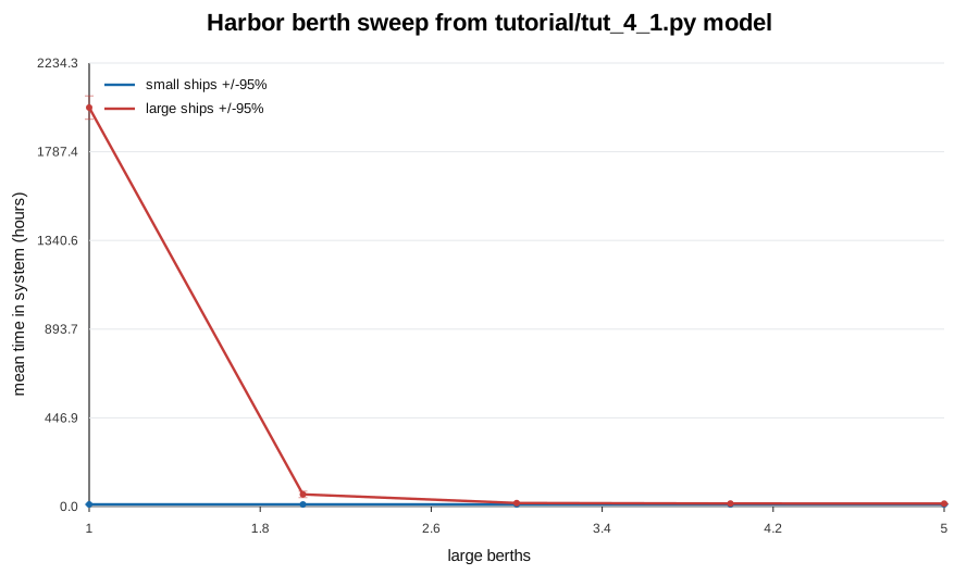
The result is the kind of plot we actually wanted all along: parameter combinations along one axis, outcome values with confidence intervals along the other, and enough replications behind the points that we can say something useful.

The plot below is generated from a real Python run of the harbor model, sweeping the number of large berths from one to five with ten replications at each level:

Adding Python-powered simulation physics

Some simulations need heavier computation inside each process: movement, geometry, sensor logic, routing, forecasting, optimization, or decision rules. The Python modeling pattern is to keep the simulation process readable and put the calculation behind small numeric helper functions.

For example, an aircraft process might update position every simulated minute, call a helper that computes detections, tally the count, and hold until the next observation time.

The AWACS scenario on a single CPU

The final scenario is an airborne sensor model. The active entities might be:

an aircraft process following a patrol pattern,
target processes changing state over time,
a sensor process scheduling observations,
and a reporting process collecting detections.

The state fields hold positions, headings, target states, and counters. Random draws perturb movement, weather, detection probability, or target behavior. Events schedule observations and state changes. Numerical helper functions keep the geometry and detection calculations separate from the process choreography.

Running tutorial/tut_5_1.py currently reports the feature status directly:

$ .venv/bin/python tutorial/tut_5_1.py
CUDA/GPU simulation hooks are not exposed in cimba Python yet.

Additional manufacturing-line tutorial

The repository also includes tutorial/assembly_line.py, a standalone three-station manufacturing-line model. It shows parts moving through station inboxes, acquiring each station’s processing resource, and leaving through a finished-parts sink while the model records cycle times, wait times, utilization, throughput, and the number of parts in the system.

Run it from the repository root with plotting dependencies installed:

uv run --extra plot python tutorial/assembly_line.py

The script writes a process graph to tutorial/assembly_line_plots/.

The key lesson is the same as in every earlier chapter: active entities are processes, passive constraints are model fields, randomness comes from cimba.sim, and experiments are independent trial tables that can be swept and summarized from Python.

This is where the tutorial stops, but not where the modeling style stops. The same pattern scales from a two-process queue to a harbor to a sensor scenario: write the active entities as processes, make shared constraints explicit, collect the outputs that answer the question, and then run enough independent trials to trust the answer.