A Simple M/M/1 Queue Parallelized
In this tutorial we walk through the same development path as the Cimba C tutorial: start with a small M/M/1 queue, make it stop, reduce the logging noise, collect statistics, refactor the model into a trial function, and finally run a replicated experiment.
The Python model has the same simulated world as the C model:
an arrival process that puts customers into a queue,
a service process that gets customers from the queue,
a
cimba.Bufferrepresenting the queue length.
In queuing theory notation, M/M/1 means memoryless interarrival times,
memoryless service times, one server, and unlimited queue capacity. With arrival
rate 0.75 and service rate 1.0, utilization is rho = 0.75. The
expected number waiting in the queue is rho ** 2 / (1 - rho), or 2.25.
Arrival, Service, and the Queue
The C tutorial starts by passing a cmb_buffer pointer to two process
functions. In Python, a process target is a normal callable; any positional or
keyword arguments passed to cimba.Process are forwarded to it. A
dataclass is a convenient replacement for the C struct used later in the
original tutorial:
from dataclasses import dataclass

import cimba


@dataclass
class MM1Trial:
    arr_rate: float = 0.75
    srv_rate: float = 1.0
    duration: float = 25.0
    seed: int = 11
    avg_queue_length: float = 0.0
    arrivals: int = 0
    services: int = 0


def arrival(ctx: MM1Trial):
    mean = 1.0 / ctx.arr_rate
    while True:
        cimba.hold(cimba.exponential(mean))
        ctx.arrivals += 1
        ctx.queue.put(1)


def service(ctx: MM1Trial):
    mean = 1.0 / ctx.srv_rate
    while True:
        ctx.queue.get(1)
        cimba.hold(cimba.exponential(mean))
        ctx.services += 1
The Python cimba.exponential() argument is the distribution mean, matching
the C tutorial’s cmb_random_exponential(mean) call. For a rate lambda,
pass 1.0 / lambda.
cimba.hold() is the Python wrapper for the process hold call. It yields the
current process to the Cimba dispatcher and resumes when simulated time reaches
the scheduled wakeup. Buffer.put(1) and Buffer.get(1) are blocking
operations with the same semantics as the native buffer.
The Python setup code is shorter because cimba.Simulation owns the
event queue, random generator, and object lifecycle:
with cimba.Simulation(seed=trial.seed) as sim:
    trial.simulation = sim
    trial.queue = cimba.Buffer("Queue")
    trial.queue.start_recording()
    trial.arrival_process = cimba.Process("Arrival", arrival, trial).start()
    trial.service_process = cimba.Process("Service", service, trial).start()
    sim.schedule(end_sim, trial.duration, obj=trial)
    sim.execute()

    trial.avg_queue_length = trial.queue.history().summary().mean
There are no explicit create/initialize/terminate/destroy calls
in Python. Objects created while a simulation is active are kept alive by the
simulation and closed when the context exits.
The complete first version is in tutorial/tut_1_1.py.
Stopping a Simulation
The C tutorial schedules a native end-simulation event. Python can now do the
same shape directly with cimba.Simulation.schedule(). A scheduled Python
event receives (subject, obj) and runs at an absolute simulation time:
def end_sim(subject, ctx: MM1Trial):
    ctx.arrival_process.stop()
    ctx.service_process.stop()
    ctx.queue.stop_recording()
    ctx.simulation.clear()


with cimba.Simulation(seed=trial.seed) as sim:
    ...
    sim.schedule(end_sim, trial.duration, obj=trial)
    sim.execute()
The direct event API also exposes handles for cancellation, rescheduling,
reprioritization, metadata lookup, and cimba.wait_event() from a process.
For simple fixed-time runs where no custom callback is needed,
cimba.Simulation.stop_at() is shorter:
with cimba.Simulation(seed=12) as sim:
    cimba.Process("Ticker", ticker).start()
    sim.stop_at(3.5)
    sim.execute()
That is the version shown in tutorial/tut_1_2.py. Use a custom stopping
event or process when ending the run depends on model state or when you need to
stop recording before clearing the queue.
Setting Logging Levels
The C tutorial uses cmb_logger_user() and logger bit masks. Python currently
exposes the native logger flag controls:
cimba.logger_flags_off(cimba.LOGGER_INFO)
cimba.logger_flags_on(cimba.LOGGER_WARNING)
It does not yet expose formatted user log records with native time/process/function prefixes. The Python tutorial therefore uses normal Python state for model-level traces:
USERFLAG1 = 0x00000001


def log_user(ctx: MM1Trial, message: str, *args: object) -> None:
    if ctx.trace is not None:
        ctx.trace.append(message % args)


def arrival(ctx: MM1Trial):
    mean = 1.0 / ctx.arr_rate
    while True:
        t_ia = cimba.exponential(mean)
        log_user(ctx, "Holds for %f time units", t_ia)
        cimba.hold(t_ia)
        ctx.arrivals += 1
        log_user(ctx, "Puts one into the queue")
        ctx.queue.put(1)
See tutorial/tut_1_3.py.
Collecting and Reporting Statistics
The native buffer has a built-in time-series recorder, and the Python binding exposes it directly:
trial.queue.start_recording()
sim.execute()
trial.queue.stop_recording()
summary = trial.queue.history().summary()
trial.avg_queue_length = summary.mean
The TimeSeries.summary() result is duration-weighted. That matters for queue
lengths and utilization, where a value held for ten simulated minutes should
count ten times as much as a value held for one minute.
The C tutorial prints text histograms and correlograms from the native library. Python builds the same structured data and formats it to match the native report:
report = cimba.reporting.resource_report(trial.queue, lags=20, correlation="pacf")
print(cimba.reporting.format_report(report))
cimba.reporting.format_report() reproduces the C tutorial’s
cmb_buffer_print_report() summary and character histogram followed by the
cmb_dataset_correlogram_print() correlogram, so the text matches the C
tutorial. The docs regenerate this exact result with
docs/tools/generate_reporting_assets.py:
Buffer levels for Queue
N  1309048  Mean    2.211  StdDev    2.812  Variance    7.909  Skewness    2.589  Kurtosis    9.915
--------------------------------------------------------------------------------
( -Infinity,      0.000)   |
[     0.000,      1.750)   |##################################################
[     1.750,      3.500)   |###############=
[     3.500,      5.250)   |########=
[     5.250,      7.000)   |##=
[     7.000,      8.750)   |###=
[     8.750,      10.50)   |##-
[     10.50,      12.25)   |#-
[     12.25,      14.00)   |-
[     14.00,      15.75)   |-
[     15.75,      17.50)   |-
[     17.50,      19.25)   |-
[     19.25,      21.00)   |-
[     21.00,      22.75)   |-
[     22.75,      24.50)   |-
[     24.50,      26.25)   |-
[     26.25,      28.00)   |-
[     28.00,      29.75)   |-
[     29.75,      31.50)   |-
[     31.50,      33.25)   |-
[     33.25,      35.00)   |-
[     35.00,  Infinity )   |-
--------------------------------------------------------------------------------
           -1.0                              0.0                              1.0
--------------------------------------------------------------------------------
   1   0.953                                  |###############################-
   2   0.346                                  |###########-
   3  -0.172                            =#####|
   4   0.139                                  |####=
   5  -0.090                               =##|
   6   0.087                                  |##=
   7  -0.058                                =#|
   8   0.064                                  |##-
   9  -0.045                                -#|
  10   0.050                                  |#=
  11  -0.037                                -#|
  12   0.043                                  |#-
  13  -0.031                                -#|
  14   0.036                                  |#-
  15  -0.026                                 =|
  16   0.032                                  |#-
  17  -0.023                                 =|
  18   0.028                                  |=
  19  -0.021                                 =|
  20   0.025                                  |=
--------------------------------------------------------------------------------
The C API also has five-number printers for datasets and time series. In Python, that is a structured value:
five = cimba.reporting.five_number(trial.queue.history())
print(five)
FiveNumberSummary(min=0, q1=0, median=1, q3=3, max=35, weighted=True)
The same report object can be rendered as generated docs figures:
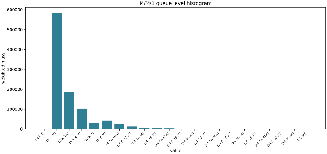
Duration-weighted queue length histogram generated by
cimba.reporting.plot_histogram().
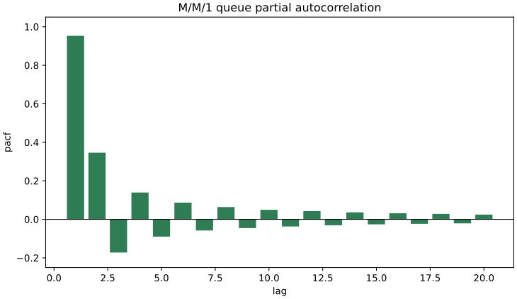
Partial autocorrelation correlogram generated by
cimba.reporting.plot_correlogram().
Theory predicts an average queue length of 2.25 at rho = 0.75. The
sample above is close enough to tell us the model is behaving plausibly, and a
longer run converges further.
Install cimba[plot] to draw the report with Matplotlib:
cimba.reporting.plot_report(report)
The warmup version, matching the C tutorial’s transition from short trace to
useful numbers, is in tutorial/tut_1_4.py.
Refactoring for Parallelism
Before parallelizing, the C tutorial moves hard-coded parameters into a
struct trial and moves the simulation driver into run_MM1_trial(). The
Python version uses the same idea:
@dataclass
class MM1Trial:
    arr_rate: float = 0.75
    srv_rate: float = 1.0
    warmup_time: float = 1000.0
    duration: float = 1.0e6
    seed: int = 123
    avg_queue_length: float = 0.0
    arrivals: int = 0
    services: int = 0


def recorder(ctx: MM1Trial):
    if ctx.warmup_time > 0.0:
        cimba.hold(ctx.warmup_time)
    ctx.queue.start_recording()
    cimba.hold(ctx.duration)
    ctx.queue.stop_recording()
    ctx.arrival_process.stop()
    ctx.service_process.stop()
    ctx.simulation.clear()


def run_mm1_trial(trial: MM1Trial) -> MM1Trial:
    with cimba.Simulation(seed=trial.seed) as sim:
        trial.simulation = sim
        trial.queue = cimba.Buffer("Queue")
        trial.arrival_process = cimba.Process("Arrival", arrival, trial).start()
        trial.service_process = cimba.Process("Service", service, trial).start()
        cimba.Process("Recorder", recorder, trial).start()
        sim.execute()

        trial.avg_queue_length = trial.queue.history().summary().mean
    return trial
This is the Python version of tutorial/tut_1_5.c and lives in
tutorial/tut_1_5.py.
Parallelization
Cimba’s parallelization strategy is the same in Python as in C at the modeling
level: run independent trials and aggregate their results. The Python API is
cimba.run_experiment(). A trial function receives (index, seed) and
returns an ordinary Python result:
def run_experiment(
    rhos=(0.25, 0.50, 0.75),
    replications=2,
    duration=2500.0,
    seed=1600,
    processes=2,
):
    rhos = tuple(rhos)
    grid = [(rho, rep) for rho in rhos for rep in range(replications)]

    def trial_fn(index, trial_seed):
        rho, rep = grid[index]
        trial = run_mm1_trial(
            MM1Trial(
                arr_rate=rho,
                srv_rate=1.0,
                duration=duration,
                seed=trial_seed,
            )
        )
        return {
            "rho": rho,
            "replication": rep,
            "avg_queue_length": trial.avg_queue_length,
        }

    samples = cimba.run_experiment(
        trial_fn,
        n=len(grid),
        seed=seed,
        processes=processes,
    )

    rows = []
    for rho in rhos:
        summary = cimba.DataSummary()
        for sample in samples:
            if sample["rho"] == rho:
                summary.add(sample["avg_queue_length"])
        rows.append({"rho": rho, "avg_queue_length": summary.mean})
    return rows
The default backend="process" is recommended for Python-defined models
because it parallelizes on ordinary GIL-enabled Python builds. The advanced
backend="thread" uses Cimba’s native pthread worker pool, but Python code
only runs in parallel there on a free-threaded interpreter.
The complete replicated example is in tutorial/tut_1_6.py. The final file,
tutorial/tut_1_7.py, adds command-line arguments in the same spirit as the
C tutorial’s final getopt version.
The upstream C tutorial plots the replicated utilization sweep like this; the
Python result rows from run_experiment() are intentionally shaped so they can
be plotted the same way:
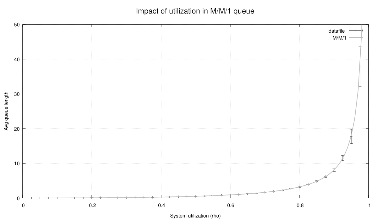
Average queue length by utilization, with confidence intervals from replicated trials.